Object Recognition with Convolutional Neural Networks

1. Introduction

In this project, we investigate into the field of machine learning and image recognition by developing a neural network model using the CIFAR-10 dataset (Krizhevsky, 2009). Our objective is to create a Convolutional Neural Network (CNN) using Keras, an open-source neural network library in Python, constructed to facilitate quick experimentation with deep neural networks.

As noted by Chollet (2015), Keras stands out for its high-level interface, providing a simpler entry point into deep learning, and its ability to operate on top of TensorFlow, a comprehensive platform for machine learning. To facilitate our development process, we will utilise Google Colab, a cloud-based Python programming environment.

This project covers critical aspects of machine learning, from data preprocessing and division of the dataset into training, validation, and testing sets, to defining the CNN architecture and fine-tuning hyperparameters. Our focus will be on preventing overfitting, ensuring model generalisation, and optimising the network’s performance.

2. Overview of the CIFAR-10 Dataset

According to Krizhevsky (2009), the CIFAR-10 dataset (Canadian Institute for Advanced Research, 10 classes) is a subset of the Tiny Images dataset and contains 60,000 32x32 colour images, gaging from animals to vehicles (see Exhibit 1).

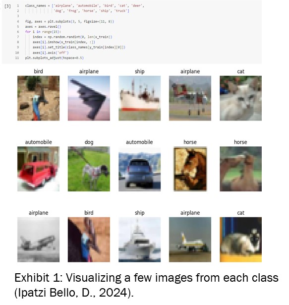
This dataset is balanced, with each class represented by 6,000 images, ensuring unbiased training for machine learning models. My detailed data analysis focused on this balance, crucial for preventing model bias (Huang et al., 2022).

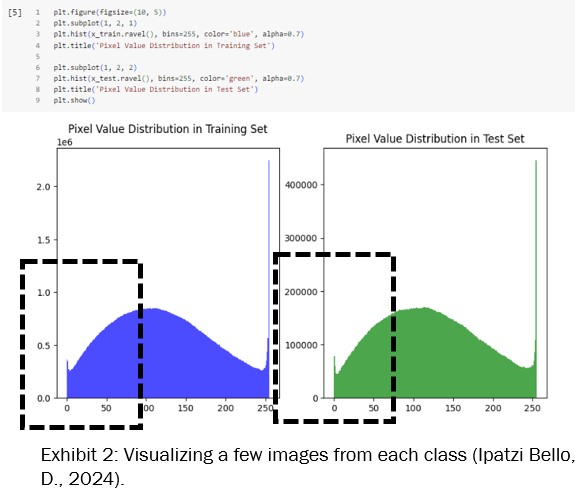
I conducted an analysis of the distribution of pixel values to gain a better understanding of the data’s structure (see Exhibit 2). By plotting histograms for both the training and test sets, I observed a consistent distribution pattern where the majority of pixel values cluster in the lower range, indicating that many images have darker pixels. This insight is particularly valuable for preprocessing steps such as normalization and can significantly influence the robustness and performance of the trained model.

The histograms for the training and test sets expose a similar distribution, which is a promising indication that the model will perform consistently on unseen data.

3. Data Preprocessing and Partitioning CIFAR-10 Dataset

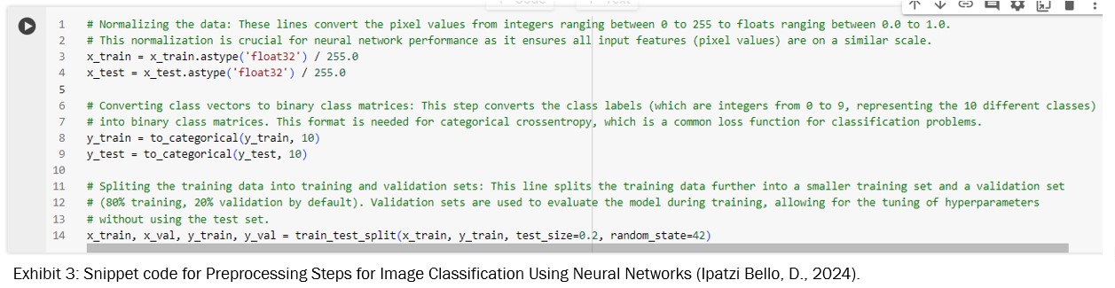
Data preprocessing is like the behind-the-scenes magic that sets up our neural network for success with the CIFAR-10 dataset. The pixel values of the dataset’s images, originally ranging from 0 to 255, go through a transformation into a floating-point format and were normalized to fall within the range of 0.0 to 1.0.

This scaling down is crucial for neural network performance as it brings uniformity to the input features, ensuring that no single pixel can excessively influence the model’s learning due to its magnitude (Huang et al., 2022).

For the class labels, they suffered a bit of a makeover too, transitioning from single digits to a fancy format called one-hot encoding (Zlateva and Rossitza Goleva, 2022, p.129). It’s more than just making things look good; it’s about getting our model to pattern with categorical cross-entropy. Think of it as the model’s way of figuring out if it’s hitting the mark or missing it, for each class.

Partitioning the dataset also played a fundamental role. The original training set was split into a new training set and a validation set, with an 80-20 split. This partitioning was carried out using the train_test_split function, which ensures that both sets are random subsets of the original.

The validation set is essential for model tuning—it acts as a proxy for the test set, allowing for the optimization of hyperparameters and providing an unbiased evaluation of the model’s performance during training.

By maintaining a separate validation set, we can iteratively improve the model and assess its generalization capability before finalizing performance. Exhibit 3 demonstrates the code snippet used for this step.

4. Designing the Neural Network

In designing the neural network, I’ve chose for a Convolutional Neural Network (CNN), recognized for its effectiveness in image classification tasks (V Kůrková et al., 2018).

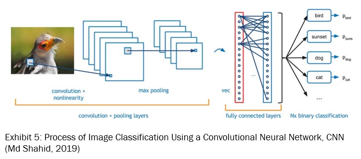
The selected architecture follows a sequential design, enabling the creation of a linear stack of layers. The CNN architecture I’ve implemented begins with convolutional layers responsible for detecting features. These layers analyse the images for patterns and details crucial for classification (see Exhibit 4).

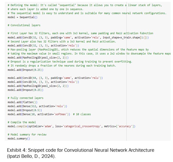
Following the convolutional layers are the pooling layers, which perform spatial down sampling to reduce the dimensionality of the feature maps, condensing the information and decreasing computational complexity.

To mitigate overfitting, dropout layers are interspersed throughout the network. These layers randomly deactivate a subset of neurons during training, assisting the network to learn more robust features that simplify better to unseen data.

At the end, the network concludes with fully connected layers, which translate the extracted features into final class predictions. Exhibit 5 illustrates the process of image classification using a CNN.

4.1 Designing the Neural Network

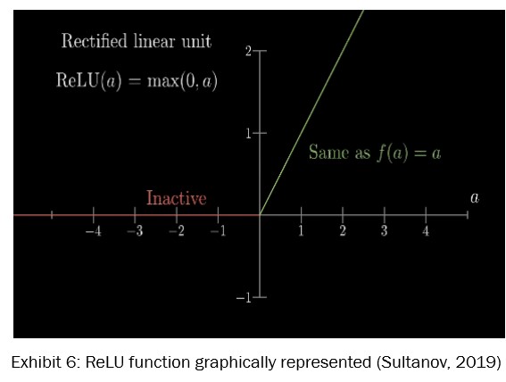
Activation functions basically take the input signal of a node in a neural network and change it into an output signal, which then gets sent to the next layer. I have selected the Rectified Linear Unit (ReLU) as the activation function. ReLU is frequently used due to its efficiency in handling non-linear data (Chen, 2021), a critical aspect for processing and classifying complex image datasets like CIFAR-10.

The ReLU function is defined mathematically as f(x) = max(0,x) and the derivative is: f’(x) = 0 if x < 0, 1 if x > 0 and thus, undefined if x = 0.

By employing the provided equation, it is evident that ReLU outputs the value x when x is positive and returns 0 otherwise. In other words, is linear for all positive values, and zero for all negative values. See please, the Exhibit 6.

In math stuff like optimization and decision-making, a loss function or cost function (sometimes even called an error function) is basically a function that turns an event or values of one or more variables into a real number (Aretz, Bartram and Pope, 2011). This number kind of shows how much “cost” is tied to that event.

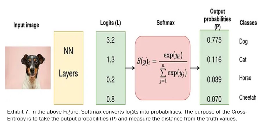
For the loss function, I implemented categorical cross entropy (also known as Softmax Loss). Lapin, Hein, and Schiele (2018) recommend this approach, which truthfully assesses the disparity between predicted probabilities and the actual distribution of classes. By employing this method, the network can refine its weights, minimizing the discrepancy between predictions and ground truth, thereby enhancing the model’s performance in managing diverse classification tasks.

In simple words, the Softmax thing takes input numbers and turns them into numbers between 0 and 1 (see Exhibit 7), like probabilities. Then it spits out a bunch of these probability numbers in a vector, one for each possible thing that could happen. And all these probabilities in the vector add up to one, covering all the possible outcomes or classes.

The combination of ReLU and categorical cross entropy aligns well with the characteristics of this dataset, facilitating an effective learning and classification process.

4.2 Model Summary Review

Our model is quite the intelligent setup. It starts with a couple of convolutional layers, which are all about recognizing those cool patterns in our images (See Exhibit 8).

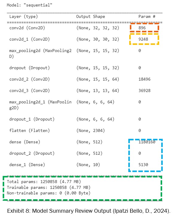
The first one comes with 896 parameters, while the second is packing a big 9,248, showing they mean business.

Then, there’s a max-pooling layer and a dropout layer tagging along, both with zero parameters but playing big roles in simplifying things and preventing the network from relying too much on the training data.

Next up, more convolution action happens, cranking up the details the network learns. And for the grand finale? Two dense layers, with the first one being a real centre featuring over a million parameters.

Totally, we’re talking about 1,250,858 trainable parameters, making this network a detailed and thoughtful way to tackle those CIFAR-10 images.

As a reminder, in neural networks, specifically (CNNs), the number of parameters reflects the network’s complexity and its ability to learn from data. More parameters usually mean that the network can capture more sophisticated patterns and details in the images.

The first few layers with fewer parameters focus on basic features like edges and colours, while deeper layers with more parameters can understand more complex and abstract patterns. This is why as we progress through the layers of our CNN, the number of parameters increases, allowing the model to learn and make more refinement distinctions between the different classes in the dataset.

5. Training the Model

The training process of our CNN model, cover 30 epochs (see Exhibit 9), showing a consistent improvement in both accuracy and loss. A lower loss indicates better performance, with the model’s predictions, being close to the actual labels.

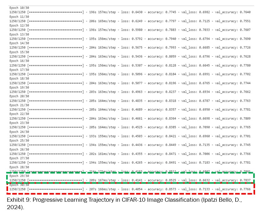
Meanwhile, the accuracy is the proportion of correctly predicted instances out of the total instances. So, higher accuracy means the model is correctly predicting more labels. Starting with an initial accuracy of around 41.75% and a loss of 1.5886 in the first epoch, the model significantly improved, reaching an accuracy of 85.73% and a loss of 0.4054 by the 30th epoch.

This progression indicates effective learning, granting there’s a signal of overfitting as the model performs better on training data compared to validation data.

Exhibit 10 offers a clear view of how the model’s performance changed throughout the training, helping in identifying the best epoch and understanding the overall training dynamics.

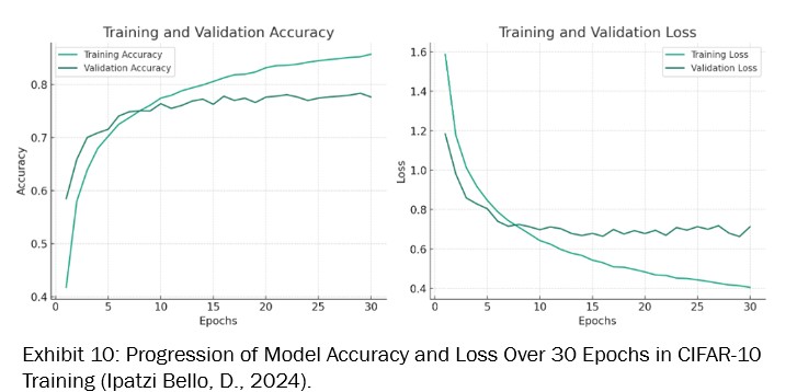
Finally, we’ve observed a consistent improvement in model performance. By the 29th epoch, the model demonstrated a robust ability to classify images, achieving a training accuracy of around 85.25% and a validation accuracy of 78.37%. The loss metrics complement this achievement, with training and validation losses recorded at 0.4405 and 0.6791, respectively.

The corresponding loss graph (see Exhibit 11) supports these findings, displaying a constant decline in both training and validation loss.

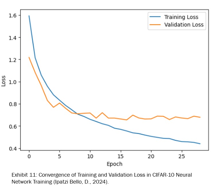
This parallel reduction is indicatory of the model’s capacity to learn and generalize effectively without significant overfitting, as evidenced by the validation loss’s stability in the final epochs.

Such a trend suggests that the model has reached a balanced state, practiced at interpreting the training data and applying its learned patterns to new, unseen data with a high degree of accuracy.

6. Model Evaluation and Results

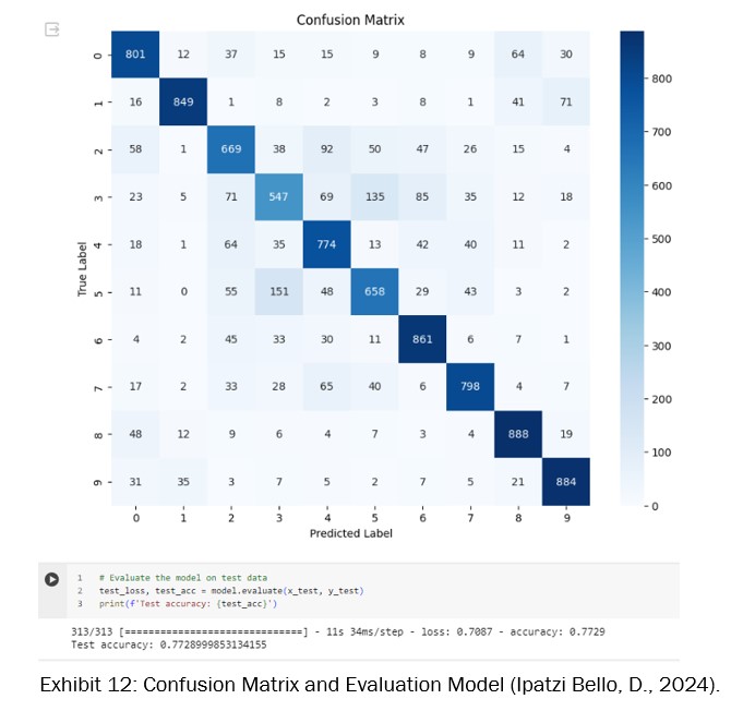
The evaluation of the neural network on the CIFAR-10 test dataset has given an accuracy of approximately 77.29% (see Exhibit 12). This performance metric indicates that the model can correctly predict the class of an image more than three-quarters of the time, which is a strong outcome for such a varied and challenging dataset.

The complementary confusion matrix provides deeper insight into the model’s performance across the ten classes. From the matrix, we can observe that classes labelled 0, 6, 8, and 9 (which could correspond to categories like airplane, frog, ship, and truck, for instance) have higher individual accuracy, with the model correctly predicting over 800 instances for each.

Some confusion is noted between classes 3 and 5 (possibly cat and dog), which is a common challenge in image classification due to the similarity between these categories.

The diagonal line of the matrix, representing correct predictions, is prominently higher than the off-diagonal elements, confirming the model’s overall strong predictive ability. This visual and numerical analysis offers valuable information, showing not only the model’s strengths but also highlighting areas where performance could be improved.

7. Challenges and Learnings

During the project, I faced various obstacles, particularly in data preprocessing, model optimization, and performance assessment. Getting the CIFAR-10 dataset ready for training demanded careful handling of pixel values and label encoding to fit the neural network architecture. Evaluating the model’s performance took a deep dive into metrics like accuracy, precision, and recall, providing valuable insights into interpreting results in image classification.

As a beginner in visual computing, the mathematics behind the models made sense, but navigating the intricacies of image processing and classification proved to be a learning curve.

While challenging, these experiences provided valuable lessons, improving my skills in data manipulation, model tuning, and result interpretation.

8. Conclusion

As a beginner in visual computing, the mathematics behind the models made sense, but navigating the intricacies of image processing and classification proved to be a learning curve.

While challenging, these experiences provided valuable lessons, improving my skills in data manipulation, model tuning, and result interpretation.

References

Aretz, K., Bartram, S.M. and Pope, P.F. (2011). Asymmetric Loss Functions and the Rationality of Expected Stock Returns. [online] mpra.ub.uni-muenchen.de. Available at: https://mpra.ub.uni-muenchen.de/47343/ [Accessed 8 Feb. 2024].

Chen, B. (2021). Why Rectified Linear Unit (ReLU) in Deep Learning and the best practice to use it with TensorFlow. [online] Medium. Available at: https://towardsdatascience.com/why-rectified-linear-unit-relu-in-deep-learning-and-the-best-practice-to-use-it-with-tensorflow-e9880933b7ef [Accessed 7 Feb. 2024].

Chollet, F. (2015). Keras documentation: About Keras. [online] keras.io. Available at: https://keras.io/about/ [Accessed 7 Feb. 2024].

Huang, Z., Sang, Y., Sun, Y. and Jiancheng Lv (2022). A neural network learning algorithm for highly imbalanced data classification. Information Sciences, 612(0020-0255), pp.496–513. doi:https://doi.org/10.1016/j.ins.2022.08.074.

Ipatzi Bello, D. (2024). Neural Network Model for Object Recognition. [online] GitHub. Available at: https://shorturl.at/jNRZ7 [Accessed 8 Feb. 2024].

Jmour, N., Zayen, S. and Abdelkrim, A. (2018). Convolutional neural networks for image classification. 2018 International Conference on Advanced Systems and Electric Technologies (IC_ASET), (978-1-5386-4449-2). doi:https://doi.org/10.1109/aset.2018.8379889.

Krizhevsky, A. (2009). The CIFAR-10 Dataset. [online] Toronto.edu. Available at: https://www.cs.toronto.edu/~kriz/cifar.html [Accessed 7 Feb. 2024].

Kubat, M. (2017). An Introduction to Machine Learning. [online] Cham: Springer International Publishing. doi:https://doi.org/10.1007/978-3-319-63913-0.

Lapin, M., Hein, M. and Schiele, B. (2018). Analysis and Optimization of Loss Functions for Multiclass, Top-k, and Multilabel Classification. IEEE Transactions on Pattern Analysis and Machine Intelligence, 40(7), pp.1533–1554. doi:https://doi.org/10.1109/tpami.2017.2751607.

Luo, T., Jiang, G., Yu, M., Zhong, C., Xu, H. and Pan, Z. (2019). Convolutional neural networks-based stereo image reversible data hiding method. Journal of Visual Communication and Image Representation, 61(1047-3203), pp.61–73. doi:https://doi.org/10.1016/j.jvcir.2019.03.017.

Md Shahid (2019). Convolutional Neural Network. Medium. Available at: https://towardsdatascience.com/covolutional-neural-network-cb0883dd6529 [Accessed 7 Feb. 2024].

Sharma, D. (2021). Image Classification Using CNN - Step-wise Tutorial. [online] Analytics Vidhya. Available at: https://www.analyticsvidhya.com/blog/2021/01/image-classification-using-convolutional-neural-networks-a-step-by-step-guide/#:~:text=CNN%20classifier%20for%20image%20classification [Accessed 6 Feb. 2024].

Sultanov, J. (2019). Magic behind Activation Function! [online] AI3 - Theory, Practice, Business. Available at: https://medium.com/ai%C2%B3-theory-practice-business/magic-behind-activation-function-c6fbc5e36a92 [Accessed 8 Feb. 2024].

Team, K. (2023). Keras documentation: CIFAR10 small images classification dataset. [online] keras.io. Available at: https://keras.io/api/datasets/cifar10/ [Accessed 6 Feb. 2024].

V Kůrková, Yannis Manolopoulos, Hammer, B., Iliadis, L.S. and Maglogiannis, I.G. (2018). Artificial neural networks and machine learning – ICANN 2018 : 27th International Conference on Artificial Neural Networks, Rhodes, Greece, October 4-7, 2018, Proceedings. Part I. Cham, Switzerland: Springer.

Zlateva, T. and Rossitza Goleva (2022). Computer Science and Education in Computer Science. Springer Nature, p.129.